【ライブラリ未使用】正規分布の累積分布関数の実装例を紹介！

この記事で解決できること

正規分布とは？
正規分布の累積分布関数の実装例
誤差計測

現実に存在する問題に対し、数値計算を用いて近似解を求めたいケースは数多く存在します。

特に、確率統計が関係する問題の場合、一般に正規分布に従うことを仮定するケースが多いです。

また、正規分布の累積分布関数を数値計算により近似的に求めることは、応用上重要なことが多いです。

そこで、今回は正規分布を題材に、プログラミングを用いて累積分布関数の近似値を求める方法を紹介します。

正規分布とは？

まずは、今回の題材である正規分布について解説します。

正規分布

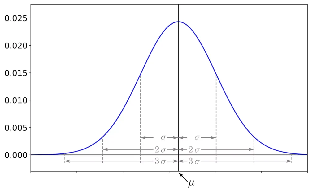
正規分布とは、データが平均付近に集積するような分布であり、確率密度関数 $f(x)$ が以下の形式で与えられる確率分布のことを指す。

$$
f(x) = \frac{1}{\sqrt{2\pi \sigma^{2}}} \exp{\left[ -\frac{(x - \mu)^{2}}{2\sigma^{2}} \right]}
$$

ここで、$\mu$ を平均、$\sigma^{2}$ を分散と呼ぶ。

特に、$\mu = 0, \sigma^{2} = 1$ の時、この分布は標準正規分布と呼ばれます。

また、正規分布に従う確率変数 $X \sim \mathcal{N}(\mu, \sigma^{2})$ を以下のように変数変換した時、この確率変数 $Z$ は標準正規分布に従います。

$$
Z = \frac{x - \mu}{\sigma}
$$

累積分布関数とは？

次に、累積分布関数について解説します。

累積分布関数（連続型確率変数の場合）

確率変数 $X$ の実現値が $x$ 以下になる関数のことで、連続型確率変数の場合、以下のように定式化される。

$$
F_{X} (x) = \int_{-\infty}^{x} f(t) \, dt
$$

※確率密度関数 $f(x)$ が存在する前提です。

正規分布の場合、累積分布関数 $F_{\mathcal{N}}(x)$ は以下のようになりますね。

$$
F_{\mathcal{N}}(x) = \int_{-\infty}^{x} \frac{1}{\sqrt{2 \pi \sigma^{2}}} \exp{\left[ -\frac{(t - \mu)^{2}}{2\sigma^{2}} \right]} \, dt
$$

正規分布の確率密度関数の実装例

以降では、正規分布の累積分布関数を求めるためのアルゴリズムと代表的なプログラミング言語による実装例を紹介します。

トピック

アルゴリズム
C言語による実装例
Javaによる実装例
javascriptによる実装例
pythonによる実装例

アルゴリズム

今回は、Handbook of Mathematical Functionsのコチラの項目を参考に実装しました。

$Z(x), x \ge 0$ を確率密度関数とすると、その累積分布関数 $P(x)$ は以下の式で近似できます。

$$
\begin{eqnarray}
P(x) & \approx & 1 - Z(x)(b_{1}t + b_{2}t^{2} + b_{3}t^{3}, b_{4}t^{4} + b_{5}t^{5}) \\
\text{ここで、} & & \\
t & = & \frac{1}{1 + px} \\
p & = & 0.2316419 \\
b_{1} & = & 0.319381530 \\
b_{2} & = & -0.356563782 \\
b_{3} & = & 1.781477937 \\
b_{4} & = & -1.821255978 \\
b_{5} & = & 1.330274429 \\
\text{である。} & &
\end{eqnarray}
$$

C言語による実装例

C言語による実装例は、以下に示す通りです。

#include <math.h>

/**
 * @brief Calculate cumulative distribution function of normal distribution
 * @param[in] x     observed value
 * @param[in] mu    mean
 * @param[in] sigma standard deviation
*/
double normalCDF(double x, double mu, double sigma) {
  const double threshold = 7.0;
  const double p  =  0.2316419;
  const double b1 =  0.319381530;
  const double b2 = -0.356563782;
  const double b3 =  1.781477937;
  const double b4 = -1.821255978;
  const double b5 =  1.330274429;
  double coef, converted, scale, pdf;
  double cdf;

  // Variable transformation of random variable
  converted = (x - mu) / sigma;
  // Validation
  if (converted < -threshold) {
    cdf = 0.0;
  }
  else if (threshold < converted) {
    cdf = 1.0;
  }
  else {
    // Calculate the value of Z(x)
    pdf = exp(-0.5 * converted * converted) / sqrt(2.0 * M_PI);
    // Calculate the value of t
    scale = 1.0 / (1.0 + fabs(converted) * p);
    // Calculate polynomial value
    coef = ((((b5 * scale + b4) * scale + b3) * scale + b2) * scale + b1) * scale;
    // Calculate the value of cumulative distribution function
    if (converted < 0) {
      cdf = pdf * coef;
    }
    else {
      cdf = 1.0 - pdf * coef;
    }
  }
  
  return cdf;
}

Javaによる実装例

Javaによる実装例は、以下に示す通りです。

class NormalDistribution {
  private double mu;
  private double sigma;
  private final double threshold = 7.0D;

  public NormalDistribution(double mu, double sigma) {
    this.mu = mu;
    this.sigma = sigma;
  }

  public double calculateNormalCDF(double x) {
    double cdf;

    // Variable transformation of random variable
    double converted = (x - mu) / sigma;
    // Validation
    if (converted < -threshold) {
      cdf = 0.0D;
    }
    else if (threshold < converted) {
      cdf = 1.0D;
    }
    else {
      double p  =  0.2316419D;
      double b1 =  0.319381530D;
      double b2 = -0.356563782D;
      double b3 =  1.781477937D;
      double b4 = -1.821255978D;
      double b5 =  1.330274429D;
      // Calculate the value of Z(x)
      double pdf = Math.exp(-0.5D * converted * converted) / Math.sqrt(2.0D * Math.PI);
      // Calculate the value of t
      double scale = 1.0D / (1.0D + Math.abs(converted) * p);
      // Calculate polynomial value
      double coef = ((((b5 * scale + b4) * scale + b3) * scale + b2) * scale + b1) * scale;
      // Calculate the value of cumulative distribution function
      if (converted < 0.0D) {
        cdf = pdf * coef;
      }
      else {
        cdf = 1.0D - pdf * coef;
      }
    }

    return cdf;
  }
}

また、Stream APIを用いる場合の実装例は、以下のようになります。

import java.util.Arrays;
import java.util.ArrayList;
import java.util.Collections;
import java.util.List;

class NormalDistribution {
  private double mu;
  private double sigma;
  private final double threshold = 7.0D;

  public NormalDistribution(double mu, double sigma) {
    this.mu = mu;
    this.sigma = sigma;
  }

  public double calculateNormalCDF(double x) {
    double cdf;

    // Variable transformation of random variable
    double converted = (x - mu) / sigma;
    // Validation
    if (converted < -threshold) {
      cdf = 0.0D;
    }
    else if (threshold < converted) {
      cdf = 1.0D;
    }
    else {
      List bs = new ArrayList<>(Arrays.asList(
         0.319381530D,
        -0.356563782D,
         1.781477937D,
        -1.821255978D,
         1.330274429D
      ));
      Collections.reverse(bs);
      double p = 0.2316419D;
      // Calculate the value of Z(x)
      double pdf = Math.exp(-0.5D * converted * converted) / Math.sqrt(2.0D * Math.PI);
      // Calculate the value of t
      double scale = 1.0D / (1.0D + Math.abs(converted) * p);
      // Calculate polynomial value
      double coef = bs.stream().reduce(0.0, (total, value) -> total * scale + value) * scale;
      // Calculate the value of cumulative distribution function
      if (converted < 0.0D) {
        cdf = pdf * coef;
      }
      else {
        cdf = 1.0D - pdf * coef;
      }
    }

    return cdf;
  }
}

javascriptによる実装例

javascriptによる実装例は、以下に示す通りです。

const normalCDF = (x, mu, sigma) => {
  const threshold = 7.0;
  const converted = (x - mu) / sigma;
  // Validation
  if (converted < -threshold) {
    return 0.0;
  }
  else if (threshold < converted) {
    return 1.0;
  }
  const p = 0.2316419;
  const bs = [0.319381530, -0.356563782, 1.781477937, -1.821255978, 1.330274429].reverse();
  const pdf = Math.exp(-0.5 * converted * converted) / Math.sqrt(2.0 * Math.PI);
  const scale = 1.0 / (1.0 + Math.abs(converted) * p);
  const coef = bs.reduce((total, current) => total * scale + current, 0.0) * scale;
  const cdf = ((converted < 0) ? (pdf * coef) : (1.0 - pdf * coef));

  return cdf;
};

pythonによる実装例

pythonによる実装例は、以下に示す通りです。

import math
import functools

def normal_cdf(x, mu, sigma):
  threshold = 7.0
  converted = (x - mu) / sigma
  cdf = 0.0

  if -threshold < converted < threshold:
    p = 0.2316419
    bs = reversed([0.319381530, -0.356563782, 1.781477937, -1.821255978, 1.330274429])
    pdf = math.exp(-0.5 * converted * converted) / math.sqrt(2.0 * math.pi)
    scale = 1.0 / (1.0 + math.fabs(converted) * p)
    coef = functools.reduce(lambda total, current: total * scale + current, bs) * scale 
    cdf = pdf * coef if converted < 0 else 1.0 - pdf * coef
  else:
    cdf = 1.0 if converted > threshold else 0.0

  return cdf

誤差計測

今回の近似式は、誤差 $\varepsilon$ が $|\varepsilon| < 7.5 \times 10^{-8} $ に収まることが知られています。

ここでは、SciPyライブラリに取り込まれているstatsというサブパッケージを用いて誤差を計測してみましょう。

今回、誤差計測に利用したコードは、以下に示す通りです。

from scipy import stats
import math
import functools
import numpy as np
import matplotlib.pyplot as plt
from scipy import stats
plt.rcParams['font.size'] = 16

def normal_cdf(x, mu, sigma):
  threshold = 7.0
  converted = (x - mu) / sigma
  cdf = 0.0

  if -threshold < converted < threshold:
    p = 0.2316419
    bs = reversed([0.319381530, -0.356563782, 1.781477937, -1.821255978, 1.330274429])
    pdf = math.exp(-0.5 * converted * converted) / math.sqrt(2.0 * math.pi)
    scale = 1.0 / (1.0 + math.fabs(converted) * p)
    coef = functools.reduce(lambda total, current: total * scale + current, bs) * scale 
    cdf = pdf * coef if converted < 0 else 1.0 - pdf * coef
  else:
    cdf = 1.0 if converted > threshold else 0.0

  return cdf

# =============
# main routine
# =============
# Calculation
mu, sigma = 0, 1
instance = stats.norm(loc=mu, scale=sigma)
xs = np.linspace(-7.1, 7.1, num=1024, endpoint=True)
_scipy_cdf = instance.cdf(xs)
_approx_cdf = np.array([normal_cdf(x, mu, sigma) for x in xs])
errs = np.abs(_scipy_cdf - _approx_cdf)

# Plot
fig, ax = plt.subplots(nrows=1, ncols=1, figsize=(10, 6))
ax.plot(xs, _scipy_cdf, '-r', label='Exact')
ax.plot(xs, _approx_cdf, '-b', label='Approx')
ax.set_xlim([xs[0], xs[-1]])
ax.legend()
# Check error
print('min: {:.9e}, max: {:.9e}'.format(errs.min(), errs.max()))

また、得られた累積分布関数のグラフを以下に示します。

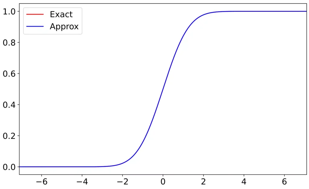
この時の誤差は、以下のようになりました。

項目	値
誤差の最小値	$8.944293022 \times 10^{-15}$
誤差の最大値	$7.450737305 \times 10^{-8}$

実用上では、問題ない程度の誤差に収まっていますね。

項目	値
誤差の最小値	\(8.944293022 \times 10^{-15}\)
誤差の最大値	\(7.450737305 \times 10^{-8}\)